Originally published by Farm and Dairy. Original article available here.

Ohio State scientist Rattan Lal wins World Food Prize

June 12, 2020

COLUMBUS, Ohio — A soil scientist at Ohio State University whose research spans five continents was awarded this year’s World Food Prize for increasing the global food supply by helping small farmers improve their soil.

Over five decades, Rattan Lal, a distinguished university professor in the College of Food, Agricultural and Environmental Sciences, has reduced hunger by pioneering agricultural methods across the globe that not only restore degraded soil but also reduce global warming.

“Every year we are astounded by the quality of nominations for the prize, but Dr. Lal’s stellar work on management and conservation of agriculture’s most cherished natural resource, the soil, set him apart,” said Gebisa Ejeta, chair of the World Food Prize Selection Committee and 2009 recipient of the award issued by the World Food Prize Foundation based in Iowa.

“The impact of his research and advocacy on sustainability of agriculture and the environment cannot be overstressed,” Ejeta said.

Big impact

Beginning in the 1970s with his research in West Africa, Lal has discovered ways to reduce deforestation, control soil erosion, and enrich soil by managing a critical element in the soil: organic carbon.

His research has provided the scientific foundation to show that soil can not only solve the global challenge of food insecurity but also global warming. As the 2020 winner of the World Food Prize announced via webcast, Lal was awarded $250,000, which he will donate for future soil research and education. He is the first at Ohio State to receive the award.

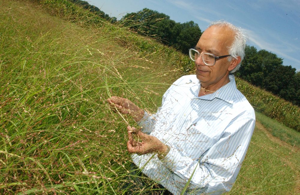
“It is a privilege and honor to be of service to the many small farmers from around the world because I was one of them. They are stewards of the land. They are the ones with the tremendous challenge of feeding the world,” said Lal, who is founding director of the Carbon Management and Sequestration Center in CFAES at Ohio State.

Lal was listed by Thomson Reuters as among the top 1% of the most-cited scientists in agriculture for the 2014 to 2019 period and among the world’s most influential scientific minds in 2015.

A faculty member at Ohio State for 33 years, Lal was recognized for his contributions to the Intergovernmental Panel on Climate Change, which shared the 2007 Nobel Peace Prize with former U.S. Vice President Al Gore.

In 2019, Lal became the first soil scientist and the first person at Ohio State to receive the Japan Prize. A year before, he received the 2018 World Agriculture Prize and the 2018 Glinka World Soil Prize.

Life story

Beyond Lal’s worldwide contributions to soil health, one of his more remarkable aspects is the trajectory of his life. At age 5, he and his family left west Punjab, resettling in northern India, as refugees, in a village without electricity. There, he and his family worked a small 7-acre farm using oxen. Drought was frequent and temperatures brutally hot. On that farm, Lal came to realize that soil can play a critical role in creating a buffer against harsh conditions by holding onto water and nutrients.

While his elder siblings ran the family farm, Lal was the only one who had a chance to go to school, the only one in his family who learned to read and write. Making the most of that opportunity, Lal pursued the education and research that have allowed him to have an impact on how policy makers and farmers across the world think about and treat soil.

In the 1990s, Lal co-wrote the first documented report showing how restoring degraded soil by taking in carbon dioxide from the air not only improved the soil but also defended against rising levels of carbon dioxide.

In the decades before and since, Lal has promoted agricultural practices that optimize the soil’s ability to act as a sponge, soaking up carbon dioxide in the air through photosynthesis, and returning it to the soil when the plant decomposes. This in turn enriches the soil, making it more conducive to growing crops.

His work

The techniques Lal has advocated include eliminating plowing, retaining crop residue left after harvest, planting cover crops, minimizing the use of chemical fertilizers, and setting aside land and water for nature, rather than for agriculture or other purposes. Each practice comes at low cost, affordable even to farmers in the developing world.

The agricultural practices Lal has promoted are now at the heart of efforts to improve agriculture systems in the tropics and globally. Lal’s research began in 1963 with studies on low corn production in India.

Working with farmers in Asia, Africa, and Latin America in the 1970s and 1980s, Lal introduced changes to the common practice of cutting down and burning swaths of trees, causing erosion of valuable topsoil. During a 10-year project that began in 2000, Lal worked with farm communities across India to promote adoption of best management practices to enhance and sustain production.

Along with his research, Lal has partnered with international and national policy makers as well as industries to increase carbon in the soil and prevent fields from eroding, keeping both sediment and chemicals from getting into nearby waterways.

All of Lal’s work has been guided by one principle: The health of soil, plants, animals, people, and the environment all depend on each other. “When the health of soil degrades, it creates a domino effect,” Lal said. “Restoring soil health is essential to restoring human health.”

Originally published by American Association for the Advancement of Science. Original article available here.

Plastic dust is blowing into U.S. national parks—more than 1000 tons each year

By Erik Stokstad Jun. 11, 2020 , 5:30 PM

Remote wilderness areas and national parks in the western United States are getting a dusting of plastic every year, perhaps 1000 tons or more, according to a new study. Up to one-quarter of the microscopic pieces of plastic—which come from carpets, clothing, and even spray paint—may originate in storms passing over nearby cities, whereas the rest likely comes from farther flung locations. The findings, the first to tease apart geographic origins, add to mounting evidence that such microplastic pollution is common worldwide.

“We created something that won’t go away,” says Janice Brahney, a biogeochemist at Utah State University and lead author on the new paper. “It’s now circulating around the globe.”

Brahney didn’t set out to track plastic pollution. Instead, she wanted to study how wind-blown dust delivers nutrients to ecosystems. So, she set up a pilot study with the National Atmospheric Deposition Program to collect such dust at a network of weather stations usually used to sample rainwater across the United States, mostly in remote locations.

Looking at samples from 11 remote areas in the western United States, including the Grand Canyon and Joshua Tree National Park, Brahney noticed brightly colored fragments under the microscope. “I realized that I was looking at deposition of plastics, which was really shocking.” Brahney didn’t have funding to study microplastic pollution, so she did the analysis on her own time, spending a “very long and stressful year” of evenings and weekends counting nearly 15,000 tiny pieces—most of them less than one-third the width of a human hair.

Brahney found a lot of tiny fibers, likely from clothes, carpets, and other textiles. She also found minuscule particles, about 30% of which were brightly colored spheres. Smaller than the plastic microbeads that have been used in cosmetics and other personal care products, the spheres are components of paints that might be released to the atmosphere during spray painting, she says.

Chelsea Rochman, an ecologist at the University of Toronto who studies microplastics, calls that finding “striking.” The paints are “a whole new source that hasn’t really been discussed before.”

The remaining 70% of the particles were harder to classify. So Brahney and a colleague turned to a technique called Fourier transform infrared spectroscopy to analyze those particles and the fibers. It showed that the samples contained on average 4% plastic. “That number blew us away,” says Brahney, who had expected less than 1%.

After running the numbers, Brahney and her colleagues estimated that about 132 pieces of microplastic land on every square meter of wilderness each day. That adds up to more than 1000 tons of plastic per year across national parks and other protected areas of the western United States—the equivalent of 300 million plastic water bottles, they report today in Science. Other studies have found similar amounts of microplastics in remote locations, including Europe’s Pyrenees Mountains and in Arctic. But the new study has far more detailed data, which helped Brahney in her next step: figuring out where the plastic was coming from.

To do that, Brahney used a weather model to identify the paths of storms for 48 hours before they reached the sampling sites. Storms that had passed over or near large cities carried more microplastic than other storms, she found. The largest amounts were carried in storms that had passed over Denver; these storms deposited 14 times as much microplastic in the Rocky Mountain National Park sample station as storms that came from other directions. The pieces of microplastic were also larger than those that settled out of the air in dry weather, suggesting the strong winds of the storms had picked up the heavier pieces.

Brahney says most of the plastic is likely coming from more distant locations, brought in via high-altitude winds rather than regional rainstorms. About 75% of the plastic was deposited during dry rather than rainy weather. Those pieces tended to be smaller—the size of extremely fine dust, which can travel for thousands of kilometers. In addition, the deposition patterns showed some influence of the jet stream. Higher elevation sites also tended to have more microplastic, further implying that the particles move high in the atmosphere—and may circulate globally.

Rochman calls this piece of the study the “wow” part. Trying to understand the patterns and processes of how microplastics move around the globe is only just beginning, she says.

Brahney is now working with atmospheric scientists who specialize in dust transport to study such questions as how plastic particles move through the atmosphere, where they might come from, and how much could be in the air. Much of this microplastic might have been circulating for years, if not decades, she says. The particles may have first settled in farm fields, or deserts, or the ocean and then have been picked up again by winds as part of a global “plastic cycle.”

Original press release available here.

Cinematic voyage across the globe’s oceans captivates and educates

The Ocean Health Voyage, an online educational platform produced by a University of Miami professor and award-winning filmmaker, is now offered to members of the Hemispheric University Consortium. 

For two years, Ali Habashi, an award-winning filmmaker and assistant professor at the University of Miami School of Communication, set off to meet with 10 world-renowned marine biologists in 10 remote locations around the globe in order to unearth stories about the health of the world’s oceans. 

Even as Habashi moved from country to country, through thrilling helicopter rides and deep-sea dives, his goal always remained clear. The project had to be more than just a visually pleasing production; it had to leave a lasting impression on his audience. 

“As a filmmaker, you always have to think about who is going to watch and the type of impact your work is going to have. There’s no point in creating something that’s going to be forgotten in a day,” said Habashi.

“When it comes to addressing challenges such as environmental or global public health issues or climate change, we need to find ways to reach all the students no matter if they’re studying at the School of Communication, College of Engineering, School of Education and Human Development, or Miami Herbert Business School. They all need to have that essential education,” he added.

“So,” Habashi continued, “part of the innovation here is to create a sustainable framework where we as communicators and filmmakers can incorporate our cinematic skillset to capture the inspiration that drives a distinguished researcher dealing with such issues in a distant location and bring that global experience to our students across the hemisphere. The new generation of students are hardly willing to settle for anything less.”

With funding from the Herbert W. Hoover Foundation, the hundreds of hours of footage Habashi collected on his journey culminated in the making of Ocean Health Voyage, an innovative educational online platform that weaves a modular syllabus with adventurous documentary-style films.

As Habashi explained, the educational cinematic experience features marine researchers on-site from field locations, above and underwater, as they teach fundamental ocean science and shine a light on the real-life complexities of working with stakeholders, finding solutions for balancing resource consumption, and conservation.

“Re-channeling the energy it takes to tackle a global film and incorporating high-caliber documentary media into an innovative online platform, which can then be experienced and meaningfully retained by a much broader scope of students, can be a turning point for those professional documentary filmmakers who are working on a global scale,” he said.  

Now, this educational platform is available to the 14 university members of the Hemispheric University Consortium (HUC). Initiated by the University of Miami in 2018 and led by President Julio Frenk, the HUC aspires to be a space “where unique partnerships are formed among equals, subject to mutual benefit and mutual accountability, where knowledge is co-constructed, and research and innovation are shared.”

With the support and leadership of each partner institution’s administration and directors of innovation, the HUC universities have now adopted this educational platform. This semester, the course went from the University of Miami to being taught at Universidad Austral in Argentina, Universidad de los Andes in Colombia, Pontificia Universidad Católica Madre y Maestra in the Dominican Republic, Universidad San Francisco de Quito in Ecuador, Tecnologico de Monterrey and Universidad de las Americas Puebla in Mexico, and Universidad Peruana Cayetano Heredia in Peru. 

As one of the major educational initiatives the HUC, Ocean Health Voyage provides real-life educational experiences for students throughout the hemisphere by taking them on virtual journeys to Chile, Brazil, New Zealand, Hong Kong, Indonesia, Netherlands, Hawaii, and various locations in the United States to learn about biodiversity, fisheries (commercial and artisanal), clean waters, climate change and carbon storage, coastal protection, port economies, iconic species, natural products, and ecotourism. 

Maria de Lourdes Dieck-Assad, the University’s vice president for hemispheric and global affairs, whose office champions the HUC, described the Ocean Health Voyage as “an innovative opportunity to collaborate and engage academic institutions throughout Latin America, the Caribbean, and Canada to mobilize their faculty and students working on issues like climate change and sustainability as one of the central pillars of the consortium,” she said.

“We are proud of the results the Ocean Health Voyage course has had in a short time fostering global collaboration to address global challenges among students and professors across the hemisphere and look forward to the valuable knowledge it will impart on a new generation of learners,” she added. 

Gabriela Geron, director of partnerships, innovation, and communications in the office of hemispheric and global affairs, agreed that Habashi “has created an incredible course that is gaining worldwide recognition for its innovation. We are proud to support this online partnership engaging with other institutions and implementing the best technologies available for international collaboration.” 

In the summer of 2019, Ocean Health Voyage was featured by Virtually Inspired, a prestigious online platform powered by Drexel Online University that showcases innovation in online learning, which in turn led to a significant national exposure.

The course presents opportunities for students in different countries to collaborate remotely on group discussions, assignments, and capstone projects specifically designed to help them develop awareness of the marine conservation issues.

The student experience across universities is entirely flexible. Even before online learning became the norm as a result of the COVID-19 pandemic, University of Miami students, together with their counterparts across the hemisphere, were learning about ocean health at a custom pace that met each school’s individual needs. 

“Each university has its own dynamics, even in terms of the date their semester starts, or unique background of the identified faculty members. In some universities, this is a fully online course where the student will log in on their own. And, in others the faculty members use this platform as a framework for their in-person teachings,” explained Habashi.

“When you are in uncharted territory, there is clearly a need for a mixture of persistence and flexibility,” he added.

José Maria Cardoso da Silva, chair of the department of geography and regional studies in the College of Arts and Sciences who is currently teaching the course at the University of Miami, pointed out that the course’s online delivery has proven to be indispensable as the world adapts to the coronavirus crisis

“During the course, students explore our relationships with the oceans. They use the videos combined with hands-on research to acquire a multidimensional view on the importance of the oceans for humanity. Because most of the materials are available online and I use a student-centered method, there was no problem transitioning the course to a remote format due to the pandemic,” he said.

Originally published by The Conversation. Original article available here.

Climate change threatens drinking water quality across the Great Lakes

This story is part of the Pulitzer Center’s nationwide Connected Coastlines reporting initiative. For more information, go to https://pulitzercenter.org/connected-coastlines-initiative.

Authors: Gabriel Filippelli, Joseph D. Ortiz

April 29, 2020

“Do Not Drink/Do Not Boil” is not what anyone wants to hear about their city’s tap water. But the combined effects of climate change and degraded water quality could make such warnings more frequent across the Great Lakes region. 

A preview occurred on July 31, 2014, when a nasty green slime – properly known as a harmful algal bloom, or HAB – developed in the western basin of Lake Erie. Before long it had overwhelmed the Toledo Water Intake Crib, which provides drinking water to nearly 500,000 people in and around the city. 

Tests revealed that the algae was producing microcystin, a sometimes deadly liver toxin and suspected carcinogen. Unlike some other toxins, microcystin can’t be rendered harmless by boiling. So the city issued a “Do Not Drink/Do Not Boil” order that set off a three-day crisis. 

Local stores soon ran out of bottled water. Ohio’s governor declared a state of emergency, and the National Guard was called in to provide safe drinking water until the system could be flushed and treatment facilities brought back on line. 

The culprit was a combination of high nutrient pollution – nitrogen and phosphorus, which stimulate the growth of algae – from sewage, agriculture and suburban runoff, and high water temperatures linked to climate change. This event showed that even in regions with resources as vast as the Great Lakes, water supplies are vulnerable to these kinds of man-made threats. 

As Midwesterners working in the fields of urban environmental health and climate and environmental science, we believe more crises like Toledo’s could lie ahead if the region doesn’t address looming threats to drinking water quality.

Vast and abused

The Great Lakes together hold 20% of the world’s surface freshwater – more than enough to provide drinking water to over 48 million people from Duluth to Chicago, Detroit, Cleveland and Toronto. But human impacts have severely harmed this precious and vital resource. 

In 1970, after a century of urbanization and industrialization around the Great Lakes, water quality was severely degraded. Factories were allowed to dump waste into waterways rather than treating it. Inadequate sewer systems often sent raw sewage into rivers and lakes, fouling the water and causing algal blooms.

Problems like these helped spur two major steps in 1972: passage of the U.S. Clean Water Act, and adoption of the Great Lakes Water Quality Agreement between the United States and Canada. Since then, many industries have been cleaned up or shut down. Sewer systems are being redesigned, albeit slowly and at great cost. 

The resulting cuts in nutrient and wastewater pollution have brought a quick decline in HABs – especially in Lake Erie, the Great Lake with the most densely populated shoreline. But new problems have emerged, due partly to shortcomings in those laws and agreements, combined with the growing effects of climate change.

Warmer and wetter

Climate change is profoundly altering many factors that affect life in the Great Lakes region. The most immediate impacts of recent climate change have been on precipitation, lake levels and water temperatures. 

Annual precipitation in the region has increased by about 5 inches over the past century. Changes in the past five years alone – the hottest five years in recorded history – have been particularly dramatic, with a series of extreme rainfall events bringing extremely high and rapidly varying water levels to the Great Lakes.

Record high precipitation in 2019 caused flooding, property damage and beachfront losses in a number of coastal communities. Precipitation in 2020 is projected to be equally high, if not higher. Some of this is due to natural variability, but certainly some is due to climate change. 

Another clear impact of climate change is a general warming of all five Great Lakes, particularly in the springtime. The temperature increase is modest and varies from year to year and place to place, but is consistent overall with records of warming throughout the region.

Lake levels continue to reach record highs or near-record highs across the basin. What problems does this cause?

Coastal erosion
Flooding
Infrastructure damage
Economic loss

Learn more—Great Lakes Quarterly Climate Impacts & Outlook report: https://mrcc.illinois.edu/pubs/docs/GL-2020Winter_Final.pdf …

More polluted runoff

Some of these climate-related changes have converged with more direct human impacts to influence water quality in the Great Lakes. 

Cleanup measures adopted back in the 1970s imposed stringent limits on large point sources of nutrient pollution, like wastewater and factories. But smaller “nonpoint” sources, such as fertilizer and other nutrients washing off farm fields and suburban lawns, were addressed through weaker, voluntary controls. These have since become major pollution sources. 

Since the mid-1990s, climate-driven increases in precipitation have carried growing quantities of nutrient runoff into Lake Erie. This rising load has triggered increasingly severe algal blooms, comparable in some ways to the events of the 1970s. Toledo’s 2014 crisis was not an anomaly.

These blooms can make lake water smell and taste bad, and sometimes make it dangerous to drink. They also have long-term impacts on the lakes’ ecosystems. They deplete oxygen, killing fish and spurring chemical processes that prime the waters of Lake Erie for larger future blooms. Low-oxygen water is more corrosive and can damage water pipes, causing poor taste or foul odors, and helps release trace metals that may also cause health problems.

So despite a half-century of advances, in many ways Great Lakes water quality is back to where it was in 1970, but with the added influence of a rapidly changing climate.

Filtering runoff

How can the region change course and build resilience into Great Lakes coastal communities? Thanks to a number of recent studies, including an intensive modeling analysis of future climate change in Indiana, which serves as a proxy for most of the region, we have a pretty good picture of what the future could look like.

As one might guess, warming will continue. Summertime water temperatures are projected to rise by about another 5 degrees Fahrenheit by midcentury, even if nations significantly reduce their greenhouse gas emissions. This will cause further declines in water quality and negatively impact coastal ecosystems. 

The analysis also projects an increase in extreme precipitation and runoff, particularly in the winter and spring. These shifts will likely bring still more nutrient runoff, sediment contaminants and sewage overflows into coastal zones, even if surrounding states hold the actual quantities of these nutrients steady. More contaminants, coupled with higher temperatures, can trigger algal blooms that threaten water supplies. 

But recent success stories point to strategies for tackling these problems, at least at the local and regional levels.

A number of large infrastructure projects are currently underway to improve stormwater management and municipal sewer systems, so that they can capture and process sewage and associated nutrients before they are transported to the Great Lakes. These initiatives will help control flooding and increase the supply of “gray water,” or used water from bathroom sinks, washing machines, tubs and showers, for uses such as landscaping.

Cities are coupling this “gray infrastructure” with green infrastructure projects, such as green roofs, infiltration gardensand reclaimed wetlands. These systems can filter water to help remove excess nutrients. They also will slow runoff during extreme precipitation events, thus recharging natural reservoirs. 

Municipal water managers are also using smart technologies and improved remote sensing methods to create near-real-time warning systems for HABs that might help avert crises. Groups like the Cleveland Water Alliance, an association of industry, government and academic partners, are working to implement smart lake technologies in Lake Erie and other freshwater environments around the globe. Finally, states including Ohioand Indiana are moving to cut total nutrient inputs into the Great Lakes from all sources, and using advanced modeling to pinpoint those sources.

Together these developments could help reduce the size of HABs, and perhaps even reach the roughly 50% reduction in nutrient runoff that government studies suggest is needed to bring them back to their minimum extent in the mid-1990s.

Short of curbing global greenhouse gas emissions, keeping communities that rely so heavily on the Great Lakes livable will require all of these actions and more.

Originally published by The Conversation. Original article available here.

Protecting Mangroves Can Protect Billions of Dollars in Global Flooding Damage Each Year

Authors: Michael Beck, Pelayo Menendez

March 10, 2020

Hurricanes and tropical storms are estimated to cost the U.S. economy more than US$50 billion yearly in damage from winds and flooding. And as these storms travel across the Atlantic, they also ravage many Caribbean nations. 

We study coastal ecosystems and how to value the natural coastal defenses provided by mangroves, marshes and coral reefs. In a new study, we map flood risks along more than 435,000 miles (700,000 kilometers) of subtropical shoreline in 59 countries around the world. 

Along these coasts, we calculate that flood risks exceed $730 billion annually in direct impacts to property. Many government agencies and insurers estimate that indirect impacts to livelihoods and other economic activity are two to three times these direct flood costs. 

We also estimate that across these 59 countries, mangroves – salt-tolerant trees that grow along tropical coastlines worldwide – reduce risk to more than 15 million people and prevent more than $65 billion in property damages every year. Mangroves do this by blocking storm surge– the rise in sea level during storms – and dampening waves, which protect people and structures near the shore. 

Battered coastlines

Tropical storms are a well-recognized hazard along many coasts. In 2019, which was an above-normal year for tropical storm activity, 90 named storms formed around the world, including 62 days with major tropical cyclones.

As one example, Hurricane Dorian devastated the northern Bahamas with sustained winds of some 185 miles per hour. Throughout its life, Dorian’s path impacted more than 17 nations and 15 U.S. states and territories, from Grenada to Newfoundland. 

And Dorian was not even the strongest cyclone of the year. That title went to Super Typhoon Halong in the Western Pacific, which steered clear of land. Many scientists predict that climate change will make these storms more intense, with a likely increase in the proportion of storms that reach Categories 4 and 5.

It would be logical to assume that countries map the flood risks from these storms, since they have to protect residents who live near coasts, along with public infrastructure such as ports, airports, wastewater treatment centers and power plants. These facilities often are built in low-lying areas around urban and suburban centers.

However, governments and businesses only develop flood risk analyses for the shorelines of highly developed nations, where people have the resources to pay for or insure against these risks. This excludes most tropical countries, where many of the world’s most vulnerable people live.

Defending shorelines

Our study was designed to quantify these flood risks worldwide and identify solutions for reducing them. We used tools that are standard in the insurance and engineering industries, along with a five-step approach for calculating expected damage, to develop high-resolution estimates of flood risk globally. Then we coupled spatially explicit hydrodynamic flood models with economics to estimate impacts to people and property.

We focused on mangroves because they are large trees that grow quickly in salt water at the edge of the coastal zone, where they form a front line of defense. Mangroves are also excellent at trapping sediments and building land. On average, land around mangroves grows vertically by 1 to 10 millimeters per year.

We generated maps summarizing the benefits that mangroves provide in 20-kilometer coastal units around the world. They show that there are 100 coastal areas where mangroves avert $100 million or more in property damages every year. These are clearly priority zones where mangrove conservation and restoration will yield highly cost-effective benefits to people, property and national budgets.

According to our estimates, the U.S., China and Taiwan receive the greatest economic benefits – protection of property – from mangroves. Vietnam, India and Bangladesh receive the greatest social benefits – protection of people. 

Mangroves as green infrastructure

Mangrove destruction has been widespread, largely because of coastal development and aquaculture. From 1980 through the early 2000s, the world lost up to 20% of existing mangrove habitat. The rate of loss has slowed but still continues, driven by urban expansion, pollution and agriculture. 

Given our findings about how valuable mangroves are for coastal protection, we believe they should be viewed as national infrastructure and made eligible for funding from hazard mitigation and disaster recovery budgets, just like other coastal defense structures. Paying for mangrove restoration can work through the same approaches that are currently used to fund engineered protective structures such as seawalls. 

Several new studies done collaboratively with Risk Management Solutions, a leading insurance risk modeling firm, show that coastal marshes and mangroves provide significant storm reduction benefits. These findings could underpin the development of innovative insurance options for natural systems. 

Examples are already being developed for coral reefs in Mexicoand across the Caribbean. Conserving mangroves where they occur together with coral reefs can multiply the flood protection benefits from habitats. 

Working with the World Bank, countries like the Philippines and Jamaica are assessing how the benefits of mangroves can be incorporated into national finances, disaster management and proposals for the U.N. Green Climate Fund, which was created in 2010 to help developing countries mitigate greenhouse gas emissions and adapt to climate change. Our work was supported by the World Bank and Germany’s International Climate Initiative to help inform solutions for nations that are most at risk.

In many places, preserving and restoring mangrove forests can be an extremely economically effective strategy for protecting coasts from tropical storm damage. As national governments and insurers grapple with disaster management costs that are growing nearly exponentially worldwide, we believe our research can create new opportunities to pay for mangrove conservation and restoration using climate adaptation, disaster risk reduction and insurance funds.

Renowned marine scientist Michael W. Beck, Ph.D., will discuss the importance of coastal conservation at a free lecture on March 4.

Beck, a research professor in the Institute of Marine Sciences at the University of California, Santa Cruz, focuses on conserving our coastlines in an effort to reduce the risks of storm surges and flooding to property, people and our planet.

Thanks to a generous grant from the Herbert W. Hoover Foundation, Beck will speak at 7 p.m. March 4 in Auditorium 101 in the Science & Nursing Building at Kent State University at Stark, 6000 Frank Ave. NW. The event is open to the public; no tickets or reservations are required.

Beck’s approach to research is multidisciplinary – across ecology, engineering and economics – in an effort to bring clear results to decision makers. A fellow of both the Fulbright Scholar Program and the Pew Marine Conservation Program, Beck worked for 20 years at The Nature Conservancy helping to establish a global marine program before being named lead marine scientist.

“Even though Stark County is a long way from the ocean, it’s important that we generate an interest in ocean biodiversity, especially as threats to that biodiversity continue to increase,” said Greg Smith, Ph.D., assistant professor of biological sciences at Kent State Stark. “There is great value in the preservation of our natural ecosystems that buffer our coastlines from damaging storms, for example. Understanding what we are losing is crucial to creating sustainable solutions for the future.”

As part of the grant from the H.W. Hoover Foundation, Kent State Stark students will travel to Florida this summer to study the Atlantic Ocean, Gulf Coast and the Everglades ecosystems, along with Smith and Robert Hamilton IV, Ph.D., associate professor of biological sciences. The grant will also support Beck’s continuing research.

“We are thankful to the H.W. Hoover Foundation for providing the means for our regional campus to collaborate with top-tier researchers,” Smith said. “It provides our students and our community with an incredible opportunity to understand the critical need of preserving our endangered marine ecosystems.”

Originally published by the Miami Herald. Original article available here.

BY HOWARD COHEN FEBRUARY 28, 2020 11:45 AM 

Florida’s persistent blue-green algae problem in waterways has already been linked to respiratory problems. 

Now, a team of researchers, led by a University of Miami neurology professor, have found that the toxin in those algae blooms can lead to amyotrophic lateral sclerosis (ALS), a debilitating and progressive neurodegnerative disease that destroys nerve cells in the brain and spinal cord.

On the positive side, the new study also found a promising advancement in the treatment of ALS, commonly known as Lou Gehrig’s Disease.

The study, published in the Journal of Neuropathology & Experimental Neurology on Feb. 20, linked a toxin produced by blue-green algae to ALS. But it also found that a naturally occurring amino acid, L-serine, could be a possible treatment to combat the painful and deadly disease that wastes away muscles.

The scientists led by the study’s first author, David Davis, UM’s neurology professor and director of the Brain Endowment Bank, included Deborah Mash, a research professor at Nova Southeastern University’s Dr. Kiran C. Patel College of Allopathic Medicine, and Paul Alan Cox, executive director of the Brain Chemistry Labs in Jackson Hole, Wyoming.

The team, working at the Behavioral Science Foundation, a research facility on the island of St. Kitts, exposed vervet monkeys to a cyanobacterial neurotoxin called BMAA that is produced by blue-green algae, which has wreaked havoc on Florida’s shores.

The monkeys began to exhibit pathological changes in their bodies similar to what happens to people’s spinal cords in the early stages of ALS. Monkeys, rather than rodents, were used because they more closely mirror how ALS develops in humans, according to Davis.

But when these vervet monkeys were fed the L-serine amino acid at the same time they were dosed with the blue-green algae toxin for 140 days, the strategy proved illuminating. These monkeys showed a reduction in ALS-like maladies in their spinal cords.

“The big message is that dietary exposure to this cyanobacterial toxin triggers ALS-type pathology, and if you include L-serine in the diet, it could slow the progression of these pathological changes,” Davis said in a statement provided by UM. “I was surprised at how close the model mirrored ALS in humans.”

Mash said the results “holds promise for identifying a cause of sporadic ALS, which accounts for 90% of all ALS cases,” in a statement provided by Brain Chemistry Labs.

“While these data provide valuable insights, we do not yet know if L-serine will improve outcomes for human patients with ALS,” added ALS expert Walter Bradley, who was also an author on the study. 

“We need to carefully continue FDA-approved clinical trials before we can recommend that L-serine be added to the neurologists’ toolbox for the treatment of ALS. However, this vervet BMAA model will be an important new tool in the quest for new drugs to treat ALS,” Bradley said in a Brain Chemistry Labs release.

This will be the “next step” in the researchers’ plans, Davis said in a UM report. “We are very curious about how BMAA affects individuals in South Florida.”

L-serine is found in soy products, sweet potatoes, eggs, meat, and some edible seaweed, according to Cognitive Vitality. L-serine is also sold as a dietary supplement. 

The new study did not specifically say consuming these foods or taking a supplement would halt the progression of ALS or make one immune from getting the disease. 

BLUE-GREEN ALGAE TOXINS

Howard Simon, founder of the Clean Okeechobee Waters Foundation, worked alongside Davis’ team. Simon, who retired as the executive director of the American Civil Liberties Union of Florida in 2018, summarized the blue-green toxic findings as such:

▪ Cyanobacteria produces an enormous number of toxins, including microcystin and BMAA (β-Methylamino- l-alanine).

▪ Microcystin has been linked to non-alcoholic liver disease and liver cancer.

▪ BMAA has been linked to neuro-degenerative diseases, including ALS, Alzheimer’s and Parkinson’s.

▪ The newest research establishes that BMAA is a cause of early stages of ALS in vervet monkeys.

“Of course, more research is needed to determine how much exposure to the cyanobacteria toxin BMAA, and over how long a period, increases the risk of neurodegenerative diseases — much like the question several decades ago: how many cigarettes will increase my risk of lung cancer?” Simon said in an email to the Miami Herald.

WHAT IS ALS?

ALS takes two forms: sporadic — the most common form accounting for between 90% to 95% of all cases — and familial, or inherited ALS, which accounts for 5% of the cases, according to the ALS Association.

Four drugs are approved by the FDA to treat ALS and there are nationwide support groups devoted to education on the disease, but there is no cure.

ALS usually strikes people between the ages of 40 and 70 and there are an estimated 16,000 Americans who have the disease at any given time, according to the ALS Association.

New York Yankees great Lou Gehrig, who died at age 37 of ALS in 1941, may be the adopted namesake of the disease that was discovered by French neurologist Jean-Martin Charcot in 1869, but other notable people also suffered from the ailment. 

These names include theoretical physicist Stephen Hawking, Baseball Hall of Fame pitcher Jim “Catfish” Hunter, Toto bassist Mike Porcaro and actor David Niven.

FLORIDA’S ‘MASSIVE’ BLUE-GREEN ALGAE PROBLEM

“This latest research advances the understanding of crippling and terminal neuro-degenerative diseases, including ALS and Alzheimer’s disease,” said Simon. “The evidence from research is mounting, and it is pointing in the same direction: cyanobacteria (commonly called blue-green algae) produces the toxin BMAA, which has been linked to Alzheimer’s — and this latest research now shows that it triggers the earliest stages of ALS in vervet monkeys.”

Simon, now a public policy advocate in Sanibel, Simon hopes the research spurs action in Gov. Ron DeSantis’ administration.

In April 2019, DeSantis named the state’s first panel to tackle what he called a “massive problem” — blue-green algae. 

Among those on the panel were researchers from Florida International University, the University of Florida, Florida Atlantic University, Florida Gulf Coast University and the Smithsonian Marine Station at Fort Pierce.

Simon says the UM-led researchers’ L-serine findings are timely today.

“This research lends greater urgency to the effort to get the Legislature to convert science into effective policies,” Simon said. “Pending legislation (Senate Bill 712, the Clean Waterways Act) needs to be strengthened with regulatory strategies to curb the pollution of Florida waters that fuels algae blooms — which in turn creates the toxin that is poisoning the people of Florida.”

Increasing the Accessibility for Characterizing Microplastics: Introducing New Application-Based and Spectral Libraries of Plastic Particles (SLoPP and SLoPP-E)

AUTHORS: Keenan Munno, Hannah De Frond, Bridget O’Donnell, and Chelsea M. Rochman

Originally published in Analytical Chemistry. Original article can be found here.

ABSTRACT: As smaller particle sizes are increasingly included in microplastic research, it is critical to chemically characterize microparticles to identify whether particles are indeed microplastics. To increase the accessibility of methods for characterizing microparticles via Raman spectroscopy, we created an application-based library of Raman spectroscopy parameters specific to microplastics based on color, morphology, and size. We also created two spectral libraries that are representative of microplastics found in environmental samples. Here, we
present SLoPP, a spectral library of plastic particles, consisting of 148 reference spectra, including a diversity of polymer types, colors, and morphologies. To account for the effects of aging on microplastics and associated changes to Raman spectra, we present a spectral library of plastic particles aged in the environment (SLoPP-E). SLoPP-E includes 113 spectra, including a diversity of types, colors, and morphologies. The microplastics used to make SLoPP-E include environmental samples obtained across a range of matrices, geographies, and time. Our libraries increase the likelihood of spectral matching for a broad range of microplastics because our libraries include plastics containing a range of additives and pigments that are not generally included in commercial libraries. When used in combination with commercial libraries of over 24 000 spectra, 63% of the top 5 matches across all particles tested (product and environmental) are from SLoPP and SLoPP-E. These tools were developed to improve the accessibility of microplastics research in response to a growing and multidisciplinary field, as well as to enhance data quality and consistency.

Originally published in Marine Biology. Original article available here.

Abstract

Corals with high levels of total lipids are known to have increased resilience potential to bleaching, and lipid class management may shed further light on why some species are more resilient to, or are able to acclimatize to, annual bleaching stress. Here, we measured the lipid class composition of three species of Caribbean corals (Porites astreoides, Porites divaricata, and Orbicella faveolata) collected in July 2009 near Puerto Morelos, Mexico (20° 50′ N, 86° 52′ W) that were experimentally bleached 2 years in a row. Our results show that single bleaching can significantly alter lipid class composition in all species, while repeated bleaching can result in stable (i.e., acclimatized) or even more altered (i.e., not acclimatized) lipid class composition depending on the species. Specifically, P. divaricata and O. faveolata both had altered lipid class composition with losses in storage lipids following single bleaching, but maintained lipid class composition following repeated bleaching stress. However, both single and repeated bleaching altered the lipid class composition in P. astreoides, with changes persisting for the 6 weeks after repeated bleaching stress. This study provides evidence that lipid class management is part of the suite of variables associated with coral resilience, that P. divaricata and O. faveolata acclimatize their lipid class management in response to repeated bleaching stress, but that P. astreoides does not. Corals like P. divaricata and O. faveolatamay, therefore, be more suitable for coral restoration efforts since they are more likely to persist under chronic repeat bleaching scenarios predicted for later this century.

Originally published by Ecology and Evolution.  Original article available here.

Evaluating the effects of large marine predators on mobile prey behavior across subtropical reef ecosystems

Lindsay M. PhenixDana TricaricoEnrique QuinteroMark E. Bond… See all authors First published: 28 November 2019 https://doi.org/10.1002/ece3.5784

Abstract

The indirect effect of predators on prey behavior, recruitment, and spatial relationships continues to attract considerable attention. However, top predators like sharks or large, mobile teleosts, which can have substantial top–down effects in ecosystems, are often difficult to study due to their large size and mobility. This has created a knowledge gap in understanding how they affect their prey through nonconsumptive effects. Here, we investigated how different functional groups of predators affected potential prey fish populations across various habitats within Biscayne Bay, FL. Using baited remote underwater videos (BRUVs), we quantified predator abundance and activity as a rough proxy for predation risk and analyzed key prey behaviors across coral reef, sea fan, seagrass, and sandy habitats. Both predator abundance and prey arrival times to the bait were strongly influenced by habitat type, with open homogenous habitats receiving faster arrival times by prey. Other prey behaviors, such as residency and risk‐associated behaviors, were potentially driven by predator interaction. Our data suggest that small predators across functional groups do not have large controlling effects on prey behavior or stress responses over short temporal scales; however, habitats where predators are more unpredictable in their occurrence (i.e., open areas) may trigger risk‐associated behaviors such as avoidance and vigilance. Our data shed new light on the importance of habitat and context for understanding how marine predators may influence prey behaviors in marine ecosystems.

1 INTRODUCTION

Top predators are characterized by some of the largest, most enigmatic, and threatened species today on Earth (Hammerschlag & Gallagher, 2017). Often occupying upper trophic tiers, predators can influence prey directly through consumption and also indirectly via the perceived risk of predation. These nonconsumptive effects can drive food‐risk trade‐offs that alter behavior, physiology, and foraging strategies in potential prey (Beauchamp, Wahl, & Johnson, 2007; Heithaus, Frid, Wirsing, & Worm, 2008; Rasher, Hoey, & Hay, 2017). In doing so, predators drive important ecosystem processes that may induce cascading effects throughout entire ecosystems (Estes et al., 2011). Despite the important roles they play in ecosystem dynamics, many populations of large predators are declining rapidly as a result of overexploitation, and habitat loss, among a myriad of other threats (Lennox, Gallagher, Ritchie, & Cooke, 2018).

While effects of apex predators are relatively well studied in terrestrial ecosystems (e.g., Suraci, Clinchy, Dill, Roberts, & Zanette, 2016), their roles in marine systems are generally less understood (e.g., Casey et al., 2017; Sandin et al., 2008). Sharks, for instance, are traditionally considered the de facto top predator in marine ecosystems, and their vulnerabilities to fishing (Gallagher, Kyne, & Hammerschlag, 2012) and general patterns of population decline (e.g., Ferretti, Worm, Britten, Heithaus, & Lotze, 2010) have reinforced the importance of understanding the implications of their removals on marine ecosystems. Often uniformly characterized as apex predators due to their size and trophic position in marine food webs (Heupel, Knip, Simpfendorfer, & Dulvy, 2014; Hussey et al., 2014), sharks may exert strong controlling influences on prey through behaviorally‐mediated, nonconsumptive processes (i.e., predation risk) (Heithaus et al., 2008; Heithaus, Wirsing, Burkholder, Thomson, & Dill, 2009). However, the degree to which sharks actually influence the behavior and physiology of prey species remains understudied and controversial (Casey et al., 2017; Roff et al., 2016; Ruppert, Travers, Smith, Fortin, & Meekan, 2013). Studies have suggested that on coral reefs, herbivorous fish reduce their feeding rates when exposed to a larger, stationary shark decoy (Catano, Barton, Boswell, & Burkepile, 2017; Madin, Gaines, & Warner, 2010; Rizzari, Frisch, Hoey, & McCormick, 2014), but it is unknown whether this acute suppression actually triggers a long‐term reduction in feeding or if it simply redistributes the prey fish to a different area. Similarly, it remains unknown how other sympatric marine teleost predators, such as barracudas (family Sphyraenidae) or morays (family Muraenidae), compare to sharks with regard to their nonconsumptive effects on prey. Nonconsumptive effects would be expected to be particularly prevalent in shallow, open ecosystems where a larger prey item’s opportunity for escape from roving, apex predators are limited (Heithaus et al., 2009), thus suggesting a potential effect of habitat complexity.

The lack of a generalizable predator effect (consistency in direction and strength) may be expected in diverse, three‐dimensional ecosystems such as coral reefs where water is clear and opportunities to shelter temporarily are extensive. These habitats provide increased visibility for and detectability of mobile, roving predators. Studies have suggested that in coral reef food webs, reef‐associated sharks and large teleosts occupy similar trophic niches (Bond et al., 2018; Frisch et al., 2016; Roff et al., 2016), which may allow for the detection of generalizable effects of predators on prey or may divert or dilute the nonconsumptive effects of species traditionally considered apex predators on larger prey species. Our knowledge of nonconsumptive effects of marine predators on prey may benefit from examining predator–prey interactions under varying environmental conditions.

An increasingly popular technique for noninvasively assessing the relative abundance and behavior of mobile fish populations, while removing diver bias, is baited remote underwater video (BRUV) surveys (Whitmarsh, Fairweather, & Huveneers, 2017). BRUVs consist of an underwater camera focused on a standardized bait source positioned in the field of view (FOV), with the unit orientated down current from the camera. Individuals attracted to the bait that swim into the FOV are “captured” on camera (Armstrong, Bagley, & Priede, 1992), providing a permanent record of observations that can be reviewed multiple times. This record improves the accuracy of the data and allows for detailed analyses such as those required for examining animal behavior. They have also been used in studies assessing predator–prey relationships (e.g., Klages, Broad, Kelaher, & Davis, 2014) and could be readily used to investigate the potential effects of marine predators on a suite of prey species, across a variety of habitats and conditions.

Here, we used BRUVs to examine the nonconsumptive effects of multiple marine predators on various mobile prey species, across the varying habitats of Biscayne Bay, Florida. We evaluated these predator–prey interactions in three ways: (a) inferring ambient risk in each habitat by quantifying relative predator abundance and foraging activity; (b) assessing habitat‐specific responses of potential prey species by measuring prey arrival (as a proxy for apprehensiveness); and (c) gauging risk‐associated behaviors of prey as well as prey residency at the bait stations (Bond et al., 2019). We hypothesized that (a) predator activity would be greater in complex habitats (Bruno, Stachowicz, & Bertness, 2003; Hutchinson, 1957); (b) prey would take longer to arrive in less complex, more open habitats due to limited shelter opportunities; (c) prey residencies would increase and the number of risk‐associated behaviors would decrease in more complex habitats (Bruno et al., 2003).

2 METHODS

2.1 Study site

This study was conducted from January 21 to August 31, 2017 in the waters of Biscayne Bay, Florida, USA, including within the boundaries of Biscayne National Park (BNP; 25°45′42.05″N, 80°11′30.44″W; Figure 1). This area extends from Key Biscayne to Key Largo and connects to the Florida Reef Tract, the third largest coral reef system worldwide. The area is defined by a mixture of coral reefs, seagrass beds, soft corals, and sand flats. Biscayne Bay is a shallow water lagoon in which a variety of habitats provide important functional, ontogenetic, and trophic value for mangrove and reef‐associated fish, including sharks and rays, as well as sea turtles and marine mammals (Serafy, Valle, Faunce, & Luo, 2007).

2.2 Baited Remove Underwater Video (BRUV) surveys

Predator–prey interactions among and between mobile elasmobranch and teleost communities were assessed throughout Biscayne Bay and Biscayne National Park using baited remote underwater video (BRUV) surveys. Each BRUV consisted of a 48‐cm tall metal pyramid frame with the sides converging at a flat, square platform (Figure 2). Additional weights (two, 0.5 kg dive weights) were added to each BRUV frame to increase stability. Each BRUV was equipped with a 100‐cm PVC bait pole, with a mesh bait bag (150 mm × 200 mm) attached at the end (via zip ties) containing ~450 g of freshly minced Spanish sardines (Sardinella spp.). High‐definition action cameras (GoPro Hero and Hero+) were secured to the square platform and positioned to face outward, with the bait bag within the estimated 160° FOV, all lights and flashing sensors on the cameras were deactivated. All footage was shot at 1,080p high‐definition at 30 frames per second.

All BRUVs were deployed from a boat and lowered to the sea floor via 30‐m ropes attached to a visible surface buoy. Deployment depths ranged from 1.3 m to 12.8 m with an average depth of 6.7 m. In‐water free‐divers were occasionally used to navigate the BRUVs away from living corals and to ensure proper orientation on the benthic substrate. BRUVs were deployed in contiguous areas in groups of three to five, spaced ~300–500 m apart, and were allowed to soak for 60 min. Deployments were focused in the following habitat types: coral reef (defined by the presence of coral colonies and structures), sea fan (defined by the presence of patchy sea fans), seagrass (defined by contiguous areas dominated by seagrass), and sand (defined by low‐rugose habitats with open sandy areas). Deployments occurred during daylight hours, between 0800 and 1330 hr. During each round of BRUV deployments, we measured depth and water temperature (°C) using a HANNA handheld probe (Hanna Instruments, HI 98193). Temperature was recorded as a control to account for any possible anomalies; average water temperature was 24.4°C across seasons. We characterized the habitat type as coral reef, sand, sea fan, or seagrass (based on 50% coverage or higher) and whether the site was inside or outside the boundaries of Biscayne National Park (a national park with varying fishing regulations, though it is not a no‐take zone nor a marine reserve).

2.3 Video analysis and variables considered

Each 60‐min video was reviewed and analyzed in real time. Analysis began once the BRUV was firmly planted in the benthos (~15–30 s) after deployment. Predators were categorized into three trophic tiers. Upper trophic predators included barracudas (Sphyraena barracuda), as well as large bodied (>2 m) mid‐water feeding sharks. Large bodied mid‐trophic predators included large benthic feeding sharks and green moray eels (Gymnothorax funebris), while small bodied mid‐trophic predators encompassed small bodied sharks (<2 m) and spotted moray eels (Gymnothorax moringa). Groupings were determined based on relative size and the presumed correlating trophic pressures they placed on the ecosystem (Bond et al., 2018; LaymanWinemiller, Arrington, & Jepsen, 2005). Seven common prey families were identified and used to measure habitat risk and risk effects: filefish (family Monacanthidae), grunts (family Haemulidae), jacks (family Carangidae), porgies (family Sparidae), rays (family Dasyatidae & Urotrygonidae), snappers (family Lutjanidae), and triggerfish (family Balistidae). These prey families were chosen due to their observed abundance in the surveyed habitats, and since they reflect a range of consumed prey items for members of the trophic levels listed above. For example, barracuda are known to be important predators of the selected families in our study region (Hansen, 2015). Large shark species found in Biscayne Bay and Florida Bay, such as blacktip (Carcharhinus limbatus), bull (Carcharhinus leucas), great hammerhead (Sphyrna mokarran), and lemon sharks (Negaprion brevirostris), retain higher trophic positions than many of the prey families and are known fish predators (Gallagher, Shiffman, Byrnes, Hammerschlag‐Peyer, & Hammerschlag, 2017; Hammerschlag, Luo, Irschick, & Ault, 2012; Matich, Heithaus, & Layman, 2011; Roemer, Gallagher, & Hammerschlag, 2016). Bonnetheads (Sphyrna turbo) and Atlantic sharpnose (Rhizoprionodon terraenovae) sharks may have varying feeding patterns, but are primarily inshore feeders with diets consisting of teleosts, crustaceans, and cephalopods (Plumlee & Wells, 2016). Similarly, grunts, jacks, and snapper have been found inside the stomachs of nurse sharks in Florida (Castro, 2000). While there is limited data on moray eel diet in our study area, work from other Caribbean areas suggests that they are piscivorous and readily consume snappers or grunts (Randall, 1967; Young & Winn, 2003).

The relative risk of each habitat where a BRUV was deployed was estimated using two predator‐focused variables: (a) predator abundance (maxNb and maxN) and (b) predator foraging activity. Predator abundance was quantified for each trophic grouping (maxNb) by tallying the number of distinctly different individuals, determined by family, sex, size, and markings, observed throughout the entire video duration (Bond et al., 2012). Additionally, a combined predator abundance was taken from each BRUV in the form of maxN, which represents the maximum number of predators, regardless of grouping, present together at one time (Bond et al., 2012). We quantified predator foraging activity rates on the bait bags by recording the number of bites from predators and whether severe damage occurred to the bag (0 = no damage, 1 = severe damage). Bait bags were categorized as “severe damage” if the bag had major lacerations or rips, or if the bag was totally removed from the pole. Nonpredatory fish also have the potential to inflict damage to the bags (i.e., triggerfish), so any instances of damage to the bags from nonpredatory fishes (ascertained via video validation) that could have confounded the detectability of our bait were not included in these analyses.

Potential responses of prey species to ambient predation risk were estimated using arrival times for each prey family (as a proxy for apprehensiveness), as well as evaluating three prey‐focused behaviors (burst swimming, schooling, and bait residency). Arrival time (s) was measured by recording the total elapsed time until the first individual from each prey family arrived on camera. Burst swimming events (defined as a short, rapid swimming behavior away from the frame; Gallagher, Brandl, & Stier, 2016; Gallagher, Lawrence, Jain‐Schlaepfer, Wilson, & Cooke, 2016) and schooling events (defined as instances where groups of five or more conspecific individuals were present; Viscido, Parrish, & Grünbaum, 2005) were recorded for the previously defined prey groups. Bait residency (sec) was evaluated for each replicate as follows: the first fish, regardless of species, to make contact with the bait was monitored until it had moved an estimated three or more body lengths distance from the bait bag (Bond et al., 2019).

2.4 Statistical analyses

Because data violated assumptions of normality and homogeneity of variance (confirmed using Shapiro–Wilk’s and Levene’s tests), we performed a zero‐inflated generalized linear model (GLM) with a negative binomial error distribution and a log‐link function to assess the ambient risk of each habitat, with habitat type and its interaction with predator functional groups specified as the independent variables and predator maxNb as the response variable. Similarly, we performed a GLM with a negative binomial error distribution on prey arrival times, with the response variable being the arrival time of prey species and the independent variables being habitat type, predator maxN, and their interaction. Instances where an individual from a prey family did not appear on the BRUV footage (i.e., not arriving) were excluded from the model. Because this resulted in low replicates for some prey fish species (e.g., rays), we did not specify prey species as an independent variable and assumed that effects of predators are generalized across all prey species. For both GLMs, we used the obtained parameters for predictions and then plotted the predicted values against the raw data to visualize both the obtained patterns and the model fit.

Predator foraging activity and prey behaviors were then visualized using a nonmetric multidimensional scaling ordination (nMDS) based on a Manhattan distance. Furthermore, a PERMANOVA was run on the same distance matrix in order to determine if habitat type, predator maximum abundance, or their interaction affected prey behavior. Finally, we analyzed correlations between predator foraging and prey risk‐associated behaviors for each habitat using a set of Spearman rank correlation analyses. All statistical analyses were performed using R Studio (R Core Team).

3 RESULTS

A total of 194 deployments were made, within a total survey area of ~15 km². Of these, 37 deployments were discarded due to the BRUV tipping over in heavy current or poor visibility, leaving a total of 157 videos (n = 157) that were used in analyses (Table 1). A total of 184 predators were recorded by the BRUVs throughout the sampling period (Table 2). Of those predators, 80 individual elasmobranchs from eight species (7 shark species, 1 ray species) were recorded, in addition to 88 barracuda and 16 moray eels. There were limited seasonal differences in maximum predator abundances (maxN) and prey arrival times across habitats, except for seagrass beds, where maximum predator abundance was substantially higher in the wet season (0.690 ± 0.0.123 individuals, mean ± SE) than in the dry season (0.091 ± 0.063). In fact, no barracudas or large bodied mid‐trophic predators were observed in seagrass habitats during the dry seasons. However, prey arrival times in seagrass beds did not differ between the two seasons.Table 1. BRUV deployments by season and habitat type

Table 2. Summary of predatory species observed on BRUVs in the present study

Predator abundances (maxNb) were significantly different among habitat types, with coral reefs having the highest average maximum number of predators per deployment (2.21 ± 2.04), followed by sea fan habitats, sand, and seagrass habitats (Table 3, Table 4). Predictions from the GLM further suggest an interaction effect between trophic level grouping and habitat. Coral reefs had the greatest mean abundance of upper trophic and large bodied mid‐trophic predators, whereas sea fan habitats had the greatest mean abundances of small bodied mid‐trophic predators (Figure 3). Prey arrival times were significantly influenced by the interactive effects of habitat and the cumulative maximum number of predators (maxN) (Table 5). Grunts, porgies, and snappers arrived comparatively early at the BRUV deployments, while stingrays arrived substantially later. The GLM revealed that the effect of maximum predator numbers in sand, sea fan, and seagrass habitats are negative and significantly different from effects of predators on coral reefs, where cumulative predator maximum number and prey arrival time were positively correlated. This is further supported by the predictions from the model, which show a steep negative relationship in sand and seagrass habitats, a nearly flat but slightly negative relationship in sea fan habitats and a positive relationship for coral reefs (Figure 4).Table 3. Mean predator abundance per BRUV deployment across the four habitat types (coral reef, sand, sea fan, and seagrass), decomposed into the different trophic levels and their combined abundance (MaxNb)

Table 4. Summary results from a zero‐inflated negative binomial generalized linear model used to test the effects of habitat type on predator abundance (maxNb) by trophic level

Note

• Significant codes: ‘***’ 0.001 ‘**’ 0.01 ‘*’ 0.05 ‘.’ 0.1.

Table 5. Summary results of a negative binomial generalized linear model of the effects of habitat type on maximum combined predator abundance (maxN)

The nMDS ordination of both predator foraging activity (i.e., number of bites) and prey behavior in response to habitat type showed little variation among habitats (Figure 5). Generalized predator foraging activity was not significantly influenced by any habitat type, although BRUVs deployed on coral reefs experienced the highest average number of predatory bites (2.211 ± 3.441 bites, mean ± SE) and instances of severe damage to the bait bag (0.263 ± 0.452 instances, mean ± SE). Prey burst swimming (4.579 ± 7.932 events) and schooling events (6.053 ± 4.801 events) also had the highest average occurrences on coral reefs when compared to sand, sea fans, and seagrass habitats (Table 6). Average prey residency at the bait was the greatest in sea fan habitats (32.211 ± 32.527 s). The PERMANOVA to test the explanatory power of habitat, predator maximum number, and their interaction on different behaviors, albeit revealing a significant habitat effect (p = .001), only explained ~10% of the variation in the data and no effect of predator maximum number or its interaction with habitat was observed. The Spearman rank correlation test showed significant correlations between predator and prey behaviors in sand, seagrass, and sea fan habitats, but not on coral reefs (Figure 6). Schooling behavior was the only one to show a positive relationship with predator maximum numbers across sand, seagrass, and sea fan habitats.

Table 6. Mean predator foraging activity (bites and severe damage) and prey response behavior (burst swimming, schooling, and residency) across four habitat types

4 DISCUSSION

Predator–prey interactions can structure marine habitats by actively changing habitat use, foraging behaviors, and food‐web dynamics (Morosinotto, Thomson, & Korpimäki, 2010). We predicted that prey fishes would be more apprehensive and thus arrive later in the field of view of the BRUV in habitats with increased predator abundance and vice versa in those with fewer predators. Our results suggest that this pattern held true only for coral reefs, where predator numbers appeared to have a negative effect on prey arrival, while in all other habitats, the two variables were positively correlated. While coral reefs offer increased structural complexity and refuge for prey, they also increase potential predation risk by obscuring prey fish’s field of view (Bond et al., 2019). These components of the habitat may provide predators with a functional advantage when hunting, thereby creating a more dangerous environment and increasing prey vigilance in these areas. Thus, the interaction between habitat features and the probability of predator detection and successful escape can result in altered prey risk‐associated behaviors and vigilance (Heithaus et al., 2009). It has been recently argued that predators may exact greater influences on prey behavior where predation risk is predictable (Creel, 2018). While we did not measure predictability of predation risk in our study, abundance of predators in certain habitats, a potential proxy for exposure, may have resulted in a pro‐active response of apprehensiveness toward the bait, although this remains speculative.

Predators are known to match prey distributions on small scales when prey is abundant (Heithaus & Dill, 2006), and, as observed in the present study, coral reefs generally contain high numbers of piscivores (Hixon & Beets, 1993), which can inversely affect prey abundance on reefs (Beukers‐Stewart, Beukers‐Stewart, & Jones, 2011). On average, grunts and snappers arrived on coral reefs and in sea fans long before any predators. Whether predation risk is “predictable” or chronic on coral reefs remains unknown, but our findings offer an interesting potential link to the predicted food‐risk effects as described in the “control of risk” hypothesis (Creel, 2018).

Animals often express their antipredator‐behaviors in high risk situations that are brief and infrequent (Lima & Bednekoff, 1999). These acute “reactive” responses are linked to areas of unpredictable predation risk (Creel, 2018). We hypothesized that potential behavioral risk effects might be highest in open areas. Interestingly, we observed faster prey arrival times in more open, homogenous habitats such as sea fans, sandy areas, and seagrass. The lack of resources in these open, plain habitats may have rendered our BRUVs a more attractive source of food, resulting in both prey and predators arriving sooner; in our study, we found that grunts and snappers were much quicker to arrive to a habitat where predators were more abundant (Nagelkerken & Velde, 2004). It is also possible that these open and homogenous habitats provide increased escape routes to prey if needed, thus making them worth the “risk.” Additionally, since predators are often transient in these habitats (Hammerschlag, Morgan, & Serafy, 2010), attacks may be less predictable. Therefore, our observed patterns for behavioral effects in these habitats may stem from a combination of resource provisioning and unpredictability of predation risk.

In general, juvenile and small bodied sharks (i.e., small mid‐trophic predators) can be found in shallow waters to minimize their own predation risk (Guttridge et al., 2012; Heupel et al., 2014). More than half of the sharks captured on the BRUVs were species that reach maximum sizes of <2 m. While it stands to reason that smaller predators induce a weaker response in prey than larger conspecifics or species (due to gape limitations), smaller mesopredators (hawkfish, Parrachirrhites arcatus) have been found to have equal nonconsumptive effects compared to larger conspecifics (Gallagher, Brandl, et al., 2016; Gallagher, Lawrence, et al., 2016). Most predators (regardless of trophic grouping) in our videos did not stay for prolonged periods of time and, as such, they represent an acute, but relatively inconsistent, pulsed source of predation risk. Finally, some small species (e.g., bonnetheads) may also have limited effects on prey because both juveniles and adults primarily feed on crabs, lobsters, and cephalopods (Bethea et al., 2007).

The extrapolation of our results beyond our study design is hindered by several caveats. Firstly, we do not know whether arrival times are truly a consequence of perceived predation risk or if they are a function of varying densities of individuals which could not be controlled. We also did not measure water currents at each of our BRUV stations, which could have affected the bait dispersal at different rates, thus changing detection potential by prey species. Furthermore, our statistical power was weakened by poor visibility (resulting in the exclusion of 37 replicates) and a category 5 hurricane, which ended data collection a bit early and thus prevented extended sampling. In future studies, dusk or night time deployments should be added to observe predator–prey interactions after dark, which may be especially important for sharks on coral reefs (Hammerschlag et al., 2017).

The role of “apex”‐predators on reefs has been brought into question in recent years (see Roff et al., 2016). While we caution overextending the results of this study to other regions, our data suggest that predators regardless of their trophic position do not significantly control mobile prey behavior on short temporal scales, across habitats. Instead, a habitat‐specific response to a consistent signal of mobile predators on reefs may result in proactive prey vigilance and subtle food‐risk trade‐offs. Specifically, less complex habitats where predators are known to patrol yet remain temporally unpredictable in their occurrence due to limited numbers and potentially wider activity areas may induce different reactive behavioral effects such as schooling and burst swimming, which, when extended over larger time scales, could have metabolic and fitness‐level impacts on prey. Taken together, these results suggest that context is important when trying to disentangle the effects of top predators on prey in costal marine habitats, and future studies should examine the interactions between mobile predators and habitat in order to link predation risk theory to observations.

ACKNOWLEDGMENTS

This work was supported by funding to Beneath the Waves from the Herbert W. Hoover Foundation, as well as from C. and M. Jones. We are grateful to M. Riera, E. Pritchard, C. Perry, R. Tricarico, Shake‐A‐Leg, and the International Seakeepers Society for their assistance with this project. This work was conducted under a Biscayne National Park permit BISC‐00076 to AJG.

CONFLICT OF INTEREST

The authors declare no competing interests.

AUTHOR CONTRIBUTIONS

A. J. G., M. E. B., and S. J. B. conceived and designed the study. L. M. P., D. T., E. Q., and A. J. G. conduced the field work. L. M. P. and S. J. B. performed the analyses. All authors contributed to writing the manuscript and gave approval.